From FASTQ to CNV calls in Julia

08 Apr, 2024

I’ve recently worked on Julia bindings for BWA, allowing to align sequencing reads (FASTA or FASTQ) to a reference genome directly from Julia. On top of this, updates to XAM.jl and BioRecordsProcessing.jl will make it possible to build end-to-end workflows in Julia, from raw reads to analysis results.

To illustrate this I will showcase online whole-genome sequencing (WGS) copy number variation (CNV) calling on a mouse kidney tumor sample.

Briefly, we need to do the following :

Read a pair of FASTQ files
Align each pair of reads to the reference genome
Count the number of read pairs aligning to a given window in the reference genome
Normalize the counts to produce a normalized (log2) coverage profile
Use an HMM to segment the profile
Visualize the results

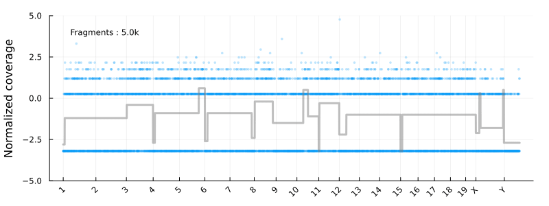
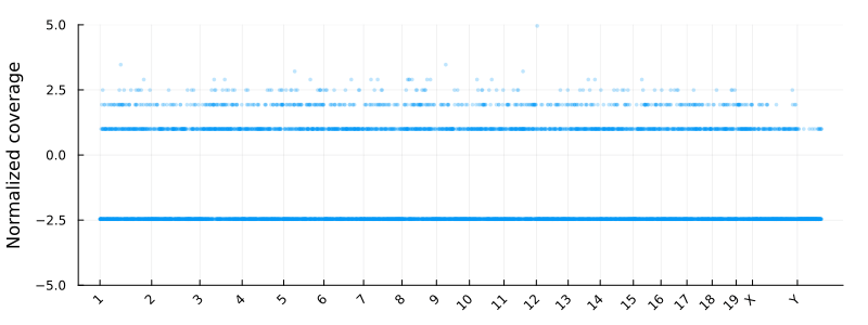
This will result in the following animation, showing how the coverage profile and segmentation evolves as more reads get processed :

targets

Disclaimer : This is not intended to be used as a serious CNV calling pipeline. I’m also using the development versions of the libraries listed above. See e.g. this article for a review of WGS CNV calling tools.

Aligning reads to the reference genome

First we need to get some data, finding publicly available WGS data from tumor is difficult, but after browsing I found this Mus musculus kidney tumor sample that has WGS data that can be downloaded from NCBI.

Next we’ll setup an aligner from BurrowsWheelerAligner.jl, loading the reference genome (which was already indexed with bwa index) :

using BurrowsWheelerAligner
const BWA = BurrowsWheelerAligner

aligner = BWA.Aligner(
    "/tmp/mouse_genome/Mus_musculus.GRCm39.dna.primary_assembly.fa.gz";
    paired = true, nthreads = 2
)

Given a pair of FASTQ reads, to obtain an alignment (as a XAM.SAM.Record) we simply do :

sam_r1, sam_r2 = BWA.align(aligner, (read1, read2))

julia>sam_r1

XAM.SAM.Record:
    template name: SRR24288063.1
            flags: 83
        reference: 13
         position: 51515489
  mapping quality: 60
...

Typically we want to save these aligned reads to a BAM file. BWA internal alignment methods returns a C string , these are parsed and wrapped in a SAM.Record, which then needs to be encoded in the proper binary representation of the BAM format. This can simply done with XAM by passing a SAM.Record to the BAM.Record constructor : XAM.BAM.Record(sam_r1).

Building a pipeline

In order to read from our pair of FASTQ files and write to a BAM file we will use BioRecordsProcessing.jl, which will do the file management for us. In BioRecordsProcessing a pipeline is built by providing a source - which will read records and pass them to a user-defined processing function - and a sink that will write the records to an output file or collect them in memory. For our case the pipeline will look like :

using BioRecordsProcessing, XAM, FASTX

file = "SRR24288063_1.fastq.gz"
header = BWA.header(aligner) # SAM.Header containing the chromosome names and lengths

p = Pipeline(
    # Source
    Reader(FASTQ, File(file; second_in_pair = x -> replace(x, "_1" => "_2"))),
    # User-defined function
    (reads...) -> begin
        r1, r2 = BWA.align(aligner, reads) 
        return BAM.Record(r1; header=header), BAM.Record(r2; header=header)
    end,
    # Sink
    Writer(
        BAM, "."; 
        extension = ".bam", header = header, paired = false
    ),
)
run(p; max_records = 2) # align two fragments

Note we passed the header when converting the records to BAM, this is needed to get the proper chromsome names in the BAM file. We can check that our BAM file is indeed correct :

run(`samtools view SRR24288063_1.fastq.bam`)
# SRR24288063.1   83      13      51515489        60      144M7S  =       51515464        -169    TTCTCTGAGCTTCA...

Counting read-pairs and coverage profile

Now that we can align our reads we want to count how many pairs fall in a given genomic interval. To do so, we define 500kb bins from chromsome 1 to chromosome Y, with the first bin of chromsome 2 following the last of chromosome 1 and so on until the end of Y :

Chr1           Chr2
-------------- -------------- ...
BIN1 BIN2 BIN3 BIN4 BIN5 BIN6

We define a function to_bin(chr, pos) taking a chromosome and genomic position to quickly compute the index of the bin corresponding to the genomic position.

chromosomes = vcat(string.(1:19), "X", "Y")

# get chromosome length from header
chromosome_lengths = [
    first(filter(h -> SAM.tag(h) == "SQ" && h["SN"] == chr, header.metainfo))["LN"] |> x->parse(Int,x)
for chr in chromosomes]

# define bins
binsize = 500_000
bins = 1:binsize:sum(chromosome_lengths)

offsets = Dict(zip(chromosomes,  vcat(0, cumsum(chromosome_lengths)[1:end-1])))
to_bin(chr, pos) = ceil(Int, (pos + offsets[chr]) / binsize)

# initialize counts to zero
counts = zeros(Int, length(bins))

We can update our processing function with:

bin_idx = to_bin(SAM.refname(r1), SAM.position(r1))
counts[bin_idx] += 1

if mod(k, 5_000) == 0
    update_plot(bins, count, offsets, anim; segmentation = nothing)
end
k += 1

Where update_plot is normalizing the counts and plot them using Plots.jl. The chromsomes are shown on the x-axis and the y axis is the log2 normalized coverage. In these coordinates -1 and 1 corresponding to copy numbers 1 and 4 for diploid cells at high tumor purity.

targets

Segmentation using a HMM

Finally we’ll use a simple hidden Markov model to segment the counts. I won’t go into details here, but shortly I’m using a fixed discretisation of the normalized coverage (from -5 to 5) for the hidden states, and a Normal emission with a standard deviation that decreases with increasing number of reads. There’s a small, uniform probability of transitioning from a hidden state to any other. Finally I use viterbi to get the most likely sequence of hidden states.

using HiddenMarkovModels, LinearAlgebra, Distributions

function segment_profile(counts)

    bins_cov = -5:0.1:5
    σ = 1/sqrt(mean(counts))

    N = length(bins_cov)
    
    p_transition = 1e-6
    transitions = I(N)*(1-p_transition) .+ p_transition
    transitions = transitions ./ sum(transitions, dims=1)

    # mix-in some uniform distributio to help with outliers
    get_emission(μ) = MixtureModel(
        vcat(Normal(μ, σ), Uniform(-5,5)), [0.99, 0.01]
    )
    emissions = [get_emission(mu) for mu in bins_cov]
    initial_state = ones(N)/N
    hmm = HMM(initial_state, transitions, emissions)

    obs_seq = log2.((counts .+ 0.1) ./ mean(counts))
    obs_seq = round.(obs_seq, digits = 1)
    obs_seq = clamp.(obs_seq, extrema(bins_cov)...)

    most_likely_state_seq, L = viterbi(hmm, obs_seq)
    seg = bins_cov[most_likely_state_seq]
    seg
end

Producing the animation shown above :

targets

Performance

Processing 10k read pairs with my pipeline takes about 30s, while simply aligning them with bwa mem took about 7 seconds, or a 4x slowdown. Both methods used 2 threads. However, profiling my Julia code indicates that most time is spent in BWA’s internal mem_process_seqs method. I’m calling this method for each read pair, it might be better to gather a batch of reads and then pass them to the method.

Final code

using BioRecordsProcessing, XAM, FASTX, BurrowsWheelerAligner, Plots, Statistics
using HiddenMarkovModels, LinearAlgebra, Distributions
const BWA = BurrowsWheelerAligner

aligner = BWA.Aligner(
    "/mnt/ssd_disk/mouse_genome/Mus_musculus.GRCm39.dna.primary_assembly.fa.gz";
    paired = true, nthreads = 2
)
header = BWA.header(aligner)

chromosomes = vcat(string.(1:19), "X", "Y")

# get chromosome length from header
chromosome_lengths = [
    first(filter(h -> SAM.tag(h) == "SQ" && h["SN"] == chr, header.metainfo))["LN"] |> x->parse(Int,x)
for chr in chromosomes]

# define bins
binsize = 500_000
bins = 1:binsize:sum(chromosome_lengths)

offsets = Dict(zip(chromosomes,  vcat(0, cumsum(chromosome_lengths)[1:end-1])))
to_bin(chr, pos) = ceil(Int, (pos + offsets[chr]) / binsize)

# initialize counts to zero
counts = zeros(Int, length(bins))

function segment_profile(counts)

    bins_cov = -5:0.1:5
    σ = 1/sqrt(mean(counts))

    N = length(bins_cov)
    
    p_transition = 1e-6
    transitions = I(N)*(1-p_transition) .+ p_transition
    transitions = transitions ./ sum(transitions, dims=1)

    get_emission(μ) = MixtureModel(
        vcat(Normal(μ, σ), Uniform(-5,5)), [0.99, 0.01]
    )
    emissions = [get_emission(mu) for mu in bins_cov]
    initial_state = ones(N)/N
    hmm = HMM(initial_state, transitions, emissions)

    obs_seq = log2.((counts .+ 0.1) ./ mean(counts))
    obs_seq = round.(obs_seq, digits = 1)
    obs_seq = clamp.(obs_seq, extrema(bins_cov)...)

    most_likely_state_seq, L = viterbi(hmm, obs_seq)
    seg = bins_cov[most_likely_state_seq]
    seg
end

function update_plot(bins, counts, offsets, anim; segmentation = nothing)
    p = scatter(
        bins, log2.((counts .+ 0.1) ./ mean(counts)), 
        alpha = 0.25, markerstrokewidth = 0, markersize = 2,
        size = (800,300), legend = false, margin = 15Plots.px,
        xticks = (values(offsets), keys(offsets)),
        xlim = extrema(bins), 
        ylim = (-5,5),
        xrotation = 45,
        ylabel = "Normalized coverage",
    )
    annotate!(bins[500], 4, text("Fragments : $(sum(counts)/1000)k", 8))
    if !isnothing(segmentation)
        sel = segmentation .!= -5
        plot!(bins[sel], segmentation[sel], c="gray", alpha = 0.5, linewidth=3)
    end
    frame(anim)
    display(p)
end

function align_fastq(aligner, file, bins, counts, max_records)
    k = 1
    anim = Animation()

    p = Pipeline(
        Reader(FASTQ, File(file; second_in_pair = x -> replace(x, "_1" => "_2"))),
        (reads...) -> begin
            r1, r2 = BWA.align(aligner, reads)
            
            !SAM.hasrefname(r1) && return nothing
            !SAM.hasrefname(r2) && return nothing
            !haskey(offsets, SAM.refname(r1)) && return nothing

            bin_idx = to_bin(SAM.refname(r1), SAM.position(r1))
            counts[bin_idx] += 1

            if mod(k, 5_000) == 0
                segmentation = segment_profile(counts)
                update_plot(bins, counts, offsets, anim; segmentation = segmentation)
            end
            k += 1

            return BAM.Record(r1; header=header), BAM.Record(r2; header=header)
        end,
        Writer(
            BAM, "."; 
            extension = ".bam", header = BWA.header(aligner), paired = false
        ),
    )
    out = run(p; max_records = max_records)
    gif(anim, "$(file)_segmentation.gif")
    out
end

file = "SRR23498664_1.fastq"

max_records = 500_000
@time align_fastq(aligner, file, bins, counts, max_records)

#Julialang #Bioinformatics